 Share This Page
| Home | | Programming Resources | | Phase-locked loops | | Share This Page |
An in-depth look at a fascinating technique
— P. Lutus — Message Page —
Copyright © 2011, P. Lutus
(double-click any word to see its definition)
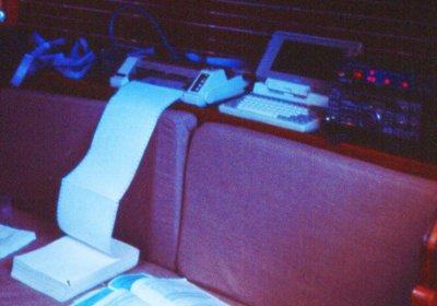
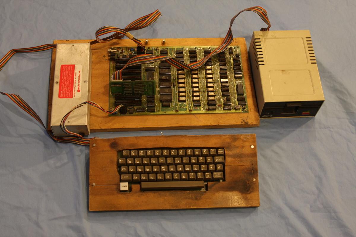
Figure 1: Printing a weather chart while underway,
somewhere in the Pacific (1988)
Detailed DescriptionThose who regularly read my technical articles may recognize the first theme I want to address — the rapid convergence of mathematics and everyday reality. In the pre-computer days of electronic technology, one would use mathematics to plan a project, then build and test a system that represented an approximate embodiment of the original math. For example, in the 1970s when I designed Space Shuttle electronics, the final flight hardware always reflected the intent of the original mathematics, but the distance between theory and practice was often large.
Now that computer methods have taken hold, in radio receiver and signal processor designs we're witnessing a rapid convergence of principles and practice. One reason is the gradual replacement of analog with digital circuits, another factor is the degree to which microprocessors now create in software what had once required explicit, single-purpose circuits. Because of the low cost and high speed of modern microprocessors, it no longer makes sense to consider most analog designs, and it's becoming practical to write signal processing code directly in software.
One of my recent projects is a software-based receiver/processor of slow-scan video images of nautical weather charts transmitted over the shortwave bands (a project named JWX). I have always needed weather charts, dating back to my around-the-world sail (1988-1991) and extending to the present, for my Alaska boat expeditions. In years past I used a demodulator box to decode shortwave weatherfax transmissions and print the result on paper (see Figure 1), but I recently realized that, because of great speed improvements, a modern laptop with a sound card should be able to perform the entire task in software, thus eliminating a single-purpose black box.
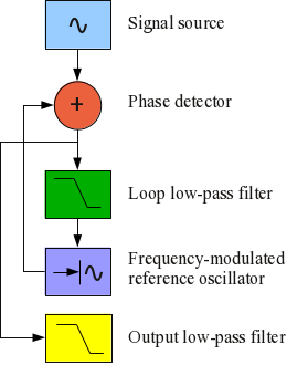
Figure 2: Phase-locked loop
block diagramIn the weatherfax project, one of the key design issues was to convert a range of audio tones into a video signal, essentially FM detection. During a lengthy design and testing phase I evaluated most known methods for FM demodulation, beginning with a crude method that counted clock cycles between zero crossings, then a system of bandpass filters, and finally I designed a phase-locked loop detector. The phase-locked loop approach turned out to be vastly superior to the other methods, to the degree that I want to describe the method in detail, so others won't pass up this terrific approach. I'll have more to say about the JWX project at the end of this article, but first let's discuss phase-locked loops.
At its most basic, a phase-locked loop (hereafter PLL) compares the frequency of a local reference oscillator to that of a received signal, and uses a feedback scheme to lock the local oscillator's frequency to the incoming signal (see Figure 2).
At this point, one application for a PLL should be obvious — the oscillator control signal's amplitude is proportional to the difference between the incoming signal's frequency and the local oscillator's free-running frequency, therefore it represents demodulated FM. But unlike typical FM detectors and with reasonable care in PLL design, the oscillator control signal can be a near-perfect duplicate of the original modulating signal, suitable for high-fidelity music, scientific telemetry, video, and other demanding requirements.
PLLs are very good FM detectors, but by changing feedback parameters, they can also detect very weak signals buried in noise — indeed a PLL is the preferred approach for detecting weak signals, as from a deep space probe. For this application the loop low-pass filter (Figure 2, green) is adjusted to allow through only a very small bandwidth (to reject noise) and the reference oscillator is tuned to the expected signal frequency. In this configuration and given adequate integration time, a PLL can detect and track a signal 40 db below accompanying noise.
I caution my readers that a PLL can't fill both the above roles at once. It can demodulate FM signals with very high accuracy and reliability, or it can detect signals buried in noise, but it can't do both in a single configuration, because the two tasks require very different setups and assumptions. In its role as an FM detector, a PLL doesn't reject noise very efficiently, and as a weak-signal detector, it can't decode FM very efficiently. The reason should be obvious — to detect FM modulation of a given bandwidth, the PLL's feedback loop low-pass filter (Figure 2, green) must be opened up enough to allow the modulation's bandwidth to pass unimpeded, but this causes the PLL to become more susceptible to noise.
Software PLL IThis section explains each block of the PLL diagram shown in Figure 2.
- Signal source
See Figure 2, blue square. It turns out that, because of how the phase detector works, the incoming signal level is critical to a PLL's performance, and in some cases one may want to consider an automatic gain control scheme. If the incoming signal drops below a certain level, the PLL will go out of lock, even in the absence of noise. If the incoming signal rises above a certain level, the possibility exists that some combinations of low-pass filter and free-running frequency settings will cause the PLL to become unstable (more on this below). The reason for these effects is that the overall feedback loop gain is proportional to the incoming signal level. Consequently, some designs may require some kind of level control, and rigorous testing under a wide range of input conditions is very desirable.- Phase detector
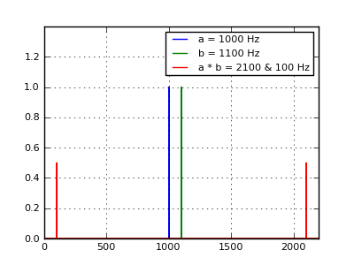
Figure 3: Phase detector analysis
See Figure 2, red circle. The most common kind of PLL phase detector is very simple — it multiplies the incoming signal and the reference oscillator signal together. For two sinewaves a and b, this is the result (see Figure 3):$a \times b = a+b\ \text{and}\ a-b$While the PLL is not in lock, in most cases it's trivial to discriminate between the a+b and a-b components (see Figure 3). Once the PLL goes into lock, once the signal and reference frequencies are the same, the low-pass filter (to be discussed next) is expected to discriminate between twice the signal/reference frequency and the expected range of modulation frequencies, which at that point will appear as amplitude variations.
I want to emphasize about the somewhat confusing Figure 3 that neither a nor b appear in the phase detector output, only a+b and a-b (only the red lines). This in essence means that, while the PLL is in lock, the low-pass filter only needs to discriminate between $2 \times a$ and the desired range of modulation frequencies.
Remember also that the modulation amplitude level present at the phase detector output represents a phase difference between the incoming and reference signals. In most cases, once that phase difference exceeds ± 90°, the PLL will go out of lock.- Loop low-pass filter
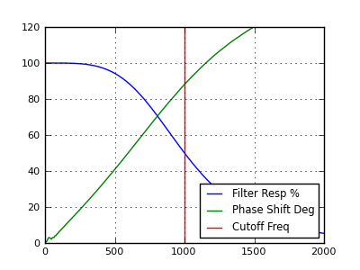
Figure 4: Low-pass filter response/phase shift
for a typical biquadratic filter
(vertical scale is both reponse %
and phase shift in degrees)See Figure 2, green square. The loop low-pass filter discriminates between twice the signal/reference frequency and the desired modulation frequencies, but it can also be used to limit the PLL lock range and susceptibility to noise. It is not uncommon that the optimal filter setting for the PLL feedback loop, and for the output signal, are different, so in many cases it is desirable to have two low-pass filters, one to set the PLL feedback loop dynamics, another to treat the output signal (Figure 2, yellow square).
A typical low-pass filter introduces some phase shift, and this has implications for feedback loop stability. In Figure 4 we see that, for a typical biquadratic low-pass filter, the phase shift at the cutoff frequency (the -3 db point) is 90°. Remember about this result that, if the PLL feedback loop gain exceeds unity at frequencies above the cutoff frequency (greater than 90° phase shift), the loop will become unstable. Read this article for more about biquadratic filters.- Frequency-modulated reference oscillator
See Figure 2, purple square. The implementation details of the reference oscillator can make or break a PLL design, but because of the flexibility of the software approach, there is little basis for comparing pure software-based and old-style analog and digital PLL designs.
The reference oscillator is essentially a frequency-modulated signal generator whose frequency is controlled by a feedback signal emanating from the phase detector / low-pass filter. So we should first study how one frequency-modulates a signal. Here is a classic FM generator equation:
(1) $\displaystyle fm(t) = \cos\left(2 \pi\ f_c\ (t + \int m(t)\ dt) \right)$Where:
- t = time, seconds
- fm(t) = frequency-modulated signal
- fc = center frequency
- m(t) = time-varying modulation signal, -1 <= m(t) <= 1
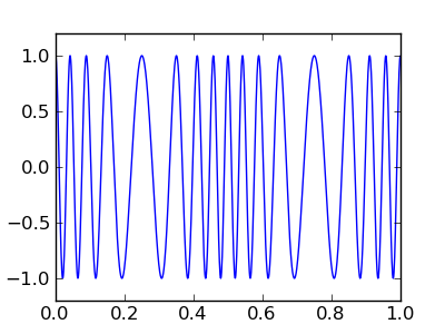
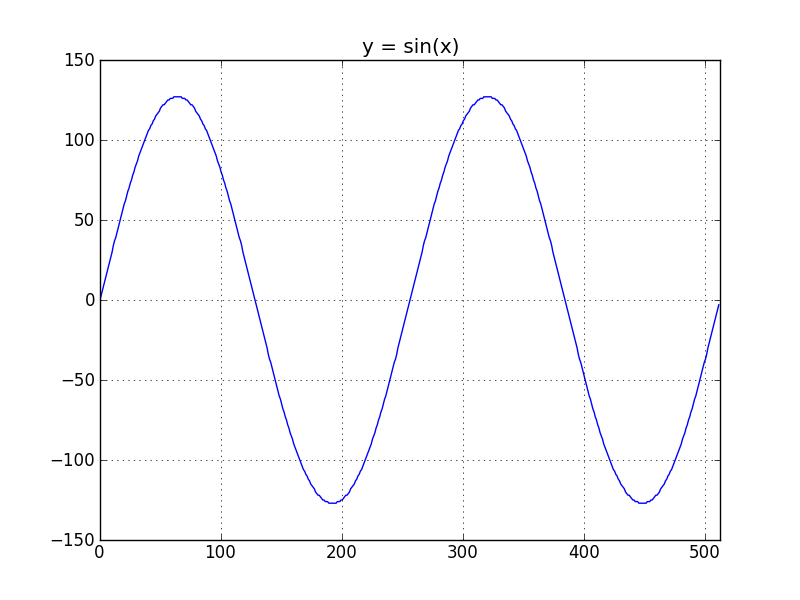
Figure 5: The result for the adjacent code
Don't be intimidated by the integral sign in equation (1) above — a practical embodiment is quite simple. Below is a complete Python program listing that solves the above equation — it generates an FM signal and plots the result (click here for plain-text source):
#!/usr/bin/env python
# -*- coding: utf-8 -*-

from pylab import *

sample_rate = 1000.0

cf = 16 # carrier frequency
mf = 2 # modulation frequency

mod_index = .5 # modulation index
fm_int = 0 # FM integral

dt = []
dfm = []

for n in range(int(sample_rate)):
  t = n / sample_rate # time seconds
  mod = cos(2 * pi * mf * t) # modulation
  fm_int += mod * mod_index / sample_rate # modulation integral
  fm = cos(2 * pi * cf * (t + fm_int)) # generate FM signal
  dt.append(t)
  dfm.append(fm)

plot(dt,dfm)
ylim(-1.2,1.2)
gcf().set_size_inches(4,3)
savefig('simple_fm_generator.png')
show()
In just a few lines, this listing produces what would be the most difficult part of a conventional (non-software) PLL design — a well-defined, controllable reference oscillator with few practical limitations. It also shows the advantage of the software design approach over the analog and integrated-circuit approaches — using the older methods, achieving the above result would lie somewhere between difficult and impossible.
Also, because it's the model for all subsequent programs in this article, note the details of the program listing. The basic idea is that a counter represents small slices of time and governs the conversion process. This arrangement is fundamental to modern signal processing, where (in a practical software radio) an analog-to-digital (A/D) converter is the signal source, delivering signal samples on a regular time schedule, and the "sample rate" referenced in the above listing is the A/D converter's clock rate.
- Output low-pass filter
See Figure 2, yellow square. As mentioned earlier, it is often desirable to treat the feedback loop dynamics and the output differently. For example, one may wish to adjust the loop low-pass filter (Figure 2, green box) to allow the PLL to aggressively track a fast-changing video signal, but filter the output signal using a different profile, one that might prevent the PLL from successfully tracking the input signal if there was just one filter. The output low-pass filter isn't essential to the operation of the PLL, but it often produces a more acceptable result.
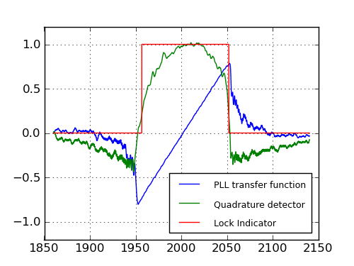
Figure 6: PLL medium sweep-frequency test
Software PLL IIIn this section we will evaluate a typical software PLL with medium bandwidth, using an example written in Python.
- Click here for a plain-text Python source file for this section's program.
- Click here for a required additional module used to create the biquadratic filters.
This example generates a frequency-sweep test signal, mixes in some noise for realism, then applies the test signal to a phase-locked loop. (The horizontal scale of Figure 6 is the frequency of the test signal.) With respect to Figure 6:
When the incoming signal's frequency equals the PLL free-running frequency, the PLL will be in lock, and there will be a 90° difference between the signal and the PLL reference oscillator. This in turn means the loop control average level is zero. If we need to detect the signal's presence and level, we need to produce a derivative of the PLL reference oscillator, shifted by 90° (a "quadrature reference") and perform another phase detection with this derived reference. The quadrature reference can be acquired with a difference equation:
- The blue trace is the PLL transfer function, the PLL loop control signal that represents the demodulated FM signal. Note that within the lock range (from 1950 to 2050 Hz) it is perfectly straight, showing that it essentially duplicates the original modulation.
- The green trace is a quadrature reference (a derivative of the PLL reference oscillator shifted by 90°) multiplied by the input signal. Unlike the PLL loop control signal, the quadrature result is at a maximum at the free-running frequency (2000 Hz). In this example, the quadrature result is used to detect the signal's presence and the lock state of the PLL.
- The red trace is a logical level derived from the quadrature reference. This signal is used to unambiguously indicate the PLL lock state.
$r_q = (r[n] - r[n-1]) \frac{\text{sample rate}}{2 \pi f}$Where:
- rq = Quadrature reference
- r[n] = Present reference oscillator sample
- r[n - 1] = Prior sample
- f = Reference oscillator free-running frequency
This isn't the only way to get a quadrature reference — in a case where there are no speed or resource limitations, one can simply generate two parallel trigonometric reference signals (sin() and cos()) instead of one. That approach is easier to create and understand, but it requires more computer power.
Notice that the green trace in Figure 6 has a dome shape within the lock region. This results from the fact that the phase relationship between the signal and quadrature reference is -90° at the left border of the lock region, 0° at 2000 Hz, and +90° at the right border of the lock region.
Here is a short excerpt from the full source listing, showing the details of the PLL and quadrature code:
  pll_loop_control = test_sig * ref_sig * pll_loop_gain # phase detector
  pll_loop_control = loop_lowpass(pll_loop_control) # loop low-pass filter
  output = output_lowpass(pll_loop_control) # output low-pass filter
  pll_integral += pll_loop_control / sample_rate # FM integral
  ref_sig = cos(2 * pi * pll_cf * (t + pll_integral)) # reference signal
  quad_ref = (ref_sig-old_ref) * sample_rate / (2 * pi * pll_cf) # quadrature reference
  old_ref = ref_sig
  pll_lock = lock_lowpass(-quad_ref * test_sig) # lock sensor
  logic_lock = (0,1)[pll_lock > 0.1] # logical lock
In this excerpt, the "output" variable produces the blue trace in Figure 6, "pll_lock" produces the green trace, and "logic_lock" produces the red trace.
This example has shown a typical PLL application — a relatively narrow, well-defined lock range, a low-pass filter set up to minimize the effect of noise, and an essentially perfect linear response in the lock range.
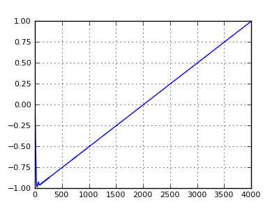
Figure 7: PLL wide sweep-frequency test
Software PLL IIIIn this section we will evaluate a software PLL with very wide bandwidth.
- Click here for a plain-text Python source file for this section's program.
- Click here for a required additional module used to create the biquadratic filters.
This example is meant to show that a PLL can be configured to have very wide lock bandwidth, if the communications channel has little noise and the signal has consistent amplitude. Figure 7 shows the transfer function for this example. The test signal (frequency on the horizontal axis) is swept from 0 Hz to 4,000 Hz, and the PLL remains locked to the input signal in the range 100 — 4000 Hz.
Notice in Figure 7 that the PLL loop control signal is perfectly linear over the entire lock range. This is expected in a PLL, but it may come as a surprise to those who have wrestled with other kinds of FM detectors.
An examination of the Python source reveals some surprising things about this example, for example there is no loop lowpass filter, only an output lowpass filter, and the loop gain is set to 8.0. One might expect such a high loop gain to cause instability, but the absence of a loop filter and its associated phase shift prevents this.
This example represents one extreme of possible PLL configurations, meant to maximize lock bandwidth. It also shows how little code is required to create a PLL — in this case, only four lines.
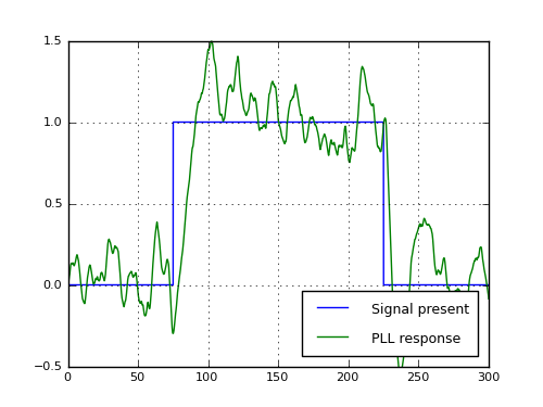
Figure 8: PLL -40db S/N signal-detection test
Application ExampleIn this section we will evaluate a software PLL with very narrow bandwidth, meant to recover a signal buried in noise.
- Click here for a plain-text Python source file for this section's program.
- Click here for a required additional module used to create the biquadratic filters.
This represents the opposite extreme of the prior example. In this example we intentionally use a very narrow acceptance bandwidth and monitor the quadrature detector's output, using a test signal with a -40 db (amplitude) signal/noise ratio. Expressed another way, in this test the noise level is 100 times the signal level.
This experiment is meant to show that a PLL can reliably detect weak signals in the presence of high noise levels. The tradeoff is that the bandwidth is restricted and the required detection time can be long. If the detected signal carries information, the data rate must be very low to avoid being overwhelmed by noise.
To get a sense of the difficulty involved in successfully detecting a signal with a -40 db signal/noise ratio, go to my signal generator page (create a separate browser tab if you can) and make the following settings:
- Signal: sine, 1000 Hz, level 1%.
- Modulation: disabled.
- Noise: level 10%.
Notice about the signal generator that you can position your mouse cursor over the controls and spin your mouse wheel to change settings — there's no need to type in numbers. And it may be necessary to increase your computer sound system's volume level to hear the generated signal.
At a signal/noise ratio of 1/10 (-20 db), a person with normal hearing can just make out the signal in the noise. Now leave the signal level at 1% and increase the noise level — increase it to 20%, then 30%. At 30% with great care, a person with excellent hearing can just make out the 1000 Hz signal. Now consider that this section's PLL example can reliably detect the signal with a 1/100 signal/noise ratio (i.e. -40db). This is why a PLL is the preferred way to detect weak signals.
In this test program, we have set a very low PLL loop filter cutoff frequency of 0.06 Hz and a loop gain of 0.00003. Remember about PLL loop dynamics that, to assure stability, a relatively low filter cutoff frequency must usually be accompanied by low loop gain.
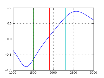
Figure 9: Biquadratic bandpass filter
detector transfer function
Reader FeedbackHere are more details about the JWX weatherfax decoder project I mentioned earlier, during which I found that a PLL was a much better FM demodulator than its alternatives. Immediately prior to considering a PLL, I had designed a system relying on biquadratic bandpass filters that did a reasonable job of demodulating the FM data from shortwave signals (see Figure 9). But there were some unsolved problems:
- An FM demodulator system using bandpass filters tends to be sensitive to amplitude as well as frequency — this is a drawback in the presence of noise.
- Because of the specifics of video detection, it's desirable to have a consistent relationship between the input signal's frequency and the output levels, regardless of the signal's amplitude. This was difficult to achieve using bandpass filters.
- It would have been nice to be able to change the frequency of the detector without having to reoptimize the filter transfer function, but this turned out to be difficult.

Figure 10: Locally-generated video test image,
demodulated by JWX after conversion to a PLL system
(Click image for full size)The PLL approach resolved all these issues, indeed once I became familiar with the methods and a handful of design principles, the system began to produce results I had not expected to achieve (see Figure 10), and that, strictly speaking, are more than adequate for shortwave weatherfax service.
Integer mathReferences
| Home | | Programming Resources | | Phase-locked loops | | Share This Page |
