Share This Page
| Home | | Mathematics | | * Sage | | | | Share This Page |
Applying Sage to physics
— P. Lutus — Message Page — Copyright © 2009, P. Lutus(double-click any word to see its definition)
To navigate this multi-page article:Use the drop-down lists and arrow icons located at the top and bottom of each page.
Click here for a copy of the
Sage worksheet used in preparing this article.
A differential equation is defined as one that makes statements about an unknown function and one or more derivatives of that function. Typically a differential equation takes the form of one or more interrelated statements about the unknown function and its derivatives. After a differential equation has been described, it might prove amenable to solution, either in closed form or by numerical modeling. It is not even a slight exaggeration to say that most of modern physics consists of a large set of differential equations and solutions.
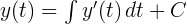
Before we play with differential equations, let's cover some preliminaries. Let's say that y(t) represents an unknown function that varies with the passage of time (t). Let's further say that the function y(t) is meant to determine a position in space. If so, then we can use this notation and these names:
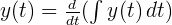
- y(t) = position
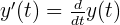
- y'(t) = velocity
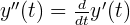
- y''(t) = acceleration
(Some may object that "velocity" should be "speed" if no direction is provided.) In this notation, y'(t) is called the "first derivative" of y(t), or y(t)'s rate of change with respect to time. And y''(t) is called the "second derivative" of y(t) — strictly speaking, y''(t) is the rate of change in y'(t) with respect to time.
This idea about rates of change is central to the Calculus of differential equations, so I'm going to expand on it a bit. If an object is located at some spatial position y(t), we can make it move by giving it a nonzero velocity (that's y'(t)). And we can change an object's velocity (y'(y)) by providing an acceleration (y''(t)).
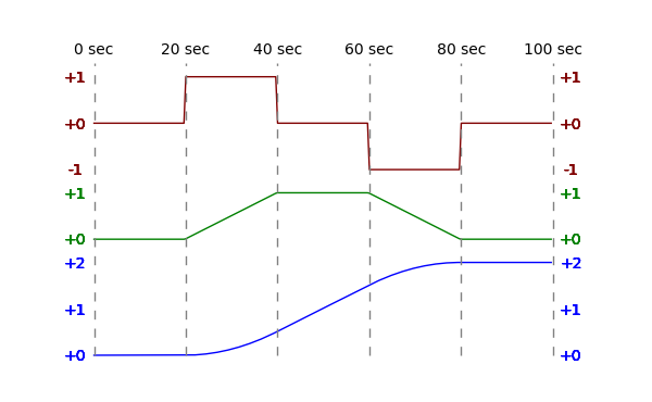
Figure 1: Relationship between acceleration, velocity and positionTake a look at Figure 1 — this chart shows how acceleration, velocity and position relate to each other. Let's say that at time 0 we're sitting in a car with the engine idling. The green velocity line (the speedometer) shows we are not moving. Then:
- At 0 seconds the car's position, velocity and acceleration are all zero.
- Because there's no acceleration, the car's velocity cannot change.
- Because there's no velocity, the car's position cannot change.
- At 20 seconds we press the accelerator pedal and the car acquires an acceleration of 1 unit.
- Because of the acceleration, over the next 20 seconds the car's velocity increases from 0 to 1 unit.
- Because of the nonzero velocity, the car begins to move.
- At 40 seconds we release the accelerator pedal and the car returns to an acceleration of zero.
- The car's velocity continues to be 1 unit.
- Because of the continuous velocity, the car moves smoothly and linearly.
- At 60 seconds we press the brake pedal and the car acquires an acceleration of -1 unit.
- Because of the deceleration, over the next 20 seconds the car's velocity decreases from 1 to 0 unit.
- Because of the decreasing velocity, the car's position changes less and finally the car stops.
- At 80 seconds we release the brake pedal and the car returns to an acceleration of zero.
- The car's velocity continues to be 0 units.
- Because of the zero velocity, the car's position no longer changes.
The car's final position differs from its starting position by 2 units. This value represents the time integral of all applied velocities, from time zero to the present. By the same token, the car's final velocity represents the time integral of all applied accelerations, from time zero to the present. This means the three quantities (acceleration, velocity and position) are interdependent. Let's explore that idea.
Integration
The relationship between acceleration, velocity and position, or any three quantities related by derivatives, lies at the heart of Calculus and of differential equations. If I have a function that describes acceleration (y''(t)), I can acquire another function that describes velocity (y'(t)) by integrating the acceleration function with respect to time:
(1)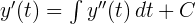
And if I have a velocity function (y'(t)), I can acquire a position function (y(t)) by integrating the velocity function with respect to time:
(2)
One can see this relationship in Figure 1 — the velocity line represents the time integral of the acceleration line, and the position line represents the time integral of the velocity line. The C term at the right of each integration represents a constant value that must be accounted for — there will be much more on this topic later on.
Differentiation
The process can be reversed — if I have a position function, I can get the equivalent velocity function by taking the position function's derivative:
(3)
And I can get the acceleration function from the velocity function in the same way:
(4)
It may occur to some of my younger readers that there is a reciprocal relationship here — one can take the derivative of a function, integrate the result, and get back the original function. This is true, and it's called the Fundamental Theorem of Calculus. Here is a very informal expression of this idea:
(5)
I apologize to the math purists among my readers for freely mixing Calculus notations from various origins. Those who want to see an overview of the different notations may read this Wikipedia article on the subject.
I want to emphasize about the above example that it's just a convenient, accessible way to show the relationship between a function y(t) and its derivatives, and position vs. time problems are only a small subset of all possible differential equations.
Let's learn how to describe and solve differential equations (DEs) with Sage. Unfortunately, as with most computer algebra systems, Sage won't allow the user to describe DEs in an intuitive way, and sometimes getting a particular result requires nothing less than sneakiness and trickery.
Sage can solve a large class of first-order and second-order Ordinary Differential Equations (ODEs) as well as Initial Value Problems (IVPs). This page is meant to show accessible solutions and methods for most common kinds of DEs, but it doesn't exhaustively detail all that Sage is capable of.
While using Sage for these examples, remember that unknown named variables must be predeclared — if a variable declaration isn't included in an example and you get an error about an undefined variable or an error message that has no obvious explanation, be sure to add a declaration for each variable that is used, like this:
var('a b c x y z')(a, b, c, x, y, z)For this first example, I'll express the differential equation using common mathematical notation, then enter it into Sage using Sage's notation. Here's the mathematical notation for our example:
(6)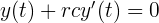 (7)
(7)
This expression says that the unknown function (the function to be found) produces the sum of y(t) and r c y'(t) for any time t, and that the initial value of the function at time zero is 1. (The meaning of r and c will become clear after a bit.) This is an example of a differential equation that specifies an initial value, as many do. In this case I intend to scale the result after acquiring the result, and this initial value makes that easy. Here is how I submit this differential equation to Sage:
var('r c t')
y = function('y',t)
de = y + r*c*diff(y,t) == 0
des = desolve(de,[y,t],[0,1]);show(des)
(8)
Let's break this entry down:
- var('r c t') tells Sage to predeclare the variables that will be used (this line isn't shown in every example).
- y = function('y',t) tells Sage that y is a function of t, e.g. as though every time I type y I mean y(t). This is a way to identify y as a function, not just a variable, and associate it with t.
- de = y + r*c*diff(y,t) == 0 creates a variable de that contains one of the statements of the DE.
- des = desolve(de,[y,t],[0,1]) invokes the Sage DE solver using our definition de as an argument, and:
- [y,t] identifies y as the function of interest and t as the dependent variable
- [0,1] sets the intial conditions: at t = 0, y = 1, or as we expressed it above, "y(0) = 1".
So it seems we were able to specify our DE to to the Sage function "desolve()" and get a result. Let's plot the result and see if it makes sense:
f(t,r,c) = des
plot(f(t,1,1),(t,0,5),figsize=(4,3))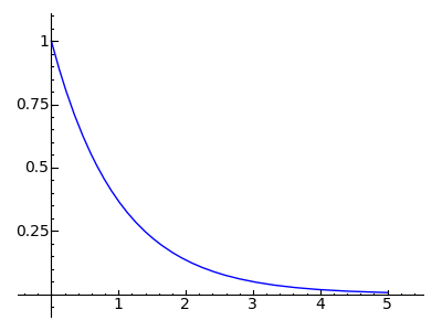
Okay, let's think about this. At time zero, y(t) equals 1. Because of how we have specified our function, y(t) + y'(t) must equal 0, or to put this another way, y'(t) = -y(t). Therefore at time zero, y'(t) (the rate of change in y(t)) is equal to -1. So y(t) begins to descend toward zero.
But as y(t) moves toward zero, something interesting happens. As the value of y(t) decreases, the rate of change also decreases (because y'(t) = -y(t)), therefore the speed with which y(t) approaches zero gradually declines. It becomes clear that the rate at which y(t) approaches zero must decline proportional to the remaining distance.
In fact, strictly speaking, y(t) only approaches zero, it never actually gets there. Doesn't this sound strange? A function that sets out for an objective but never arrives!
Isn't it nice that nature doesn't work that way? But I have a surprise for you — nature does work that way. The function we've created accurately describes a great number of natural processes, including:
- The flow of current through an electronic resistor-capacitor (RC) circuit (an identical equation appears in the linked Wikipedia article).
- The flow of heat from a hot object to a cold one (or a hot star to a cold planet).
- The flow of gas between two connected reservoirs with different pressures.
- The flow of water between two connected reservoirs with different levels.
And many other natural systems.
Let set up our function in a useful way, one that allows us to specify any starting and ending values, then we'll graph some natural processes:
f(t,a,b,r,c) = (a-b) * des + b
render("$y(t) = " + latex(f(t,a,b,r,c)) + "$","diffeq_first_example_function.png","large")
(9)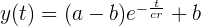
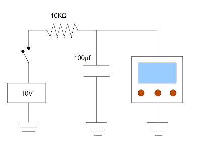
This form allows us to set any starting and ending values as well as specify the time constants r and c. Here is an example from electronics that uses the function — a plot of the voltage on a capacitor in an RC circuit to which a voltage has been applied at time zero:
# r = 10000 ohms, c = 100e-6 farads
lbl = text("$RC \, Circuit, \, r = 10000\Omega, \, c = 100\mu f $",(3,3),fontsize=12,rgbcolor='#006000')
p = plot(f(t,0,10,10000,100e-6),(t,0,5), figsize=(4,3),axes_labels=['time','v'])
show(p+lbl)
Figure 2: RC circuit test setup
(switch closes at time 0)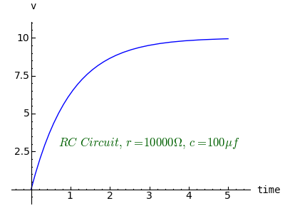
This sort of computer modeling of physical systems is becoming more common as computer power increases. It wasn't so long ago that people sat down and designed electronic circuits by throwing parts together and seeing what worked. Now it's possible to create very sophisticated models and experiment with alternatives, in advance of building an actual circuit.
This second example builds on the structure of the first — it's another equation that models a natural time delay between one event and another. But this equation, instead of modeling a one-time event like the closing of a switch, models the relationship between a continuous waveform and a dependent system. The differential equation looks like this:
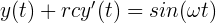
For this equation there is no initial value setting because the system being modeled is continuous. This equation models natural systems that have a driving sinusoidal waveform. Here is the process for solving it:
y = function('y',t)
de = y + r*c_t*diff(y,t) == sin(omega * t)
des = desolve(de,[y,t])
render(des,"diffeq_second_example2.png","Large")
(10)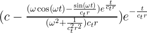
I'm showing this intermediate step in the solution so readers will understand the strategy. This class of DE is actually rather difficult to solve because initial values are assumed to exist, and it's difficult to specify the equation without any implicit or explicit initial values.
First, when the "desolve()" function doesn't get an explicit initial value specification as in this case, it automatically assigns a variable to represent it. In the result shown as equation (10) above, the initial value variable is c (and to avoid a name collision I had to rename my own time-constant c variable as ct). The c variable assigned by "desolve()" is key to creating the desired equation.
Second, notice the appearance of the e-t/ctr and et/ctr terms in the result. These are present because the DE solver wrongly assumes that an initial value is present or needed. The secret to putting this equation into the desired form is to remove these exponential terms. After some experimentation, I discovered a simple way to remove these terms — I needed to set the constant c to zero (which lifted the last constraint preventing e-t/ctr from canceling et/ctr). Like this:
des2 = (des.subs(c == 0)).full_simplify()
df(r,c_t,omega,t) = des2
render(y == df(r,c,omega,t),"diffeq_second_example3.png","Large")
(11)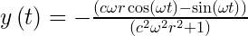
Success! Now that we've eliminated the initial-value terms, we have the canonical solution for this DE. This example, like the last, models many natural processes including resistor-capacitor circuits driven by sinusoidal waveforms, and a particular natural system of great interest to me personally — the amplitude and phase relationship between ocean tides and tides in bays. It turns out that a bay connected by a channel to the ocean has much in common with a capacitor connected by a resistor to a signal generator — both are driven by a sinusoidal waveform, and both show a predictable amplitude/phase relationship with their signal source.
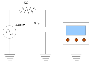
Here is a graph of an electronic test setup with a sinewave generator driving an RC circuit, much like the first example, but this time the result is continuous and a bit more complex:
# r = 1000 ohms, c = 0.5e-6 farads, f = 440
r = 1000
c = 0.5e-6
f = 440
omega = 2*pi*f
pa = plot(sin(omega*t),(t,0,.005),rgbcolor=('#800000'),axes_labels=['time','v'])
pb = plot(df(r,c,omega,t),(t,0,.005),rgbcolor=('#008000'))
lbl = text("$f = %.0f Hz \,r = %.0f \Omega \, c = %.1f {\mu}f$"
 % (f,r,c*1e6),(.0025,1.2),fontsize=12,rgbcolor='black')
show(pa+pb+lbl,figsize=(4,3))
Figure 3: RC circuit test setup (sine source)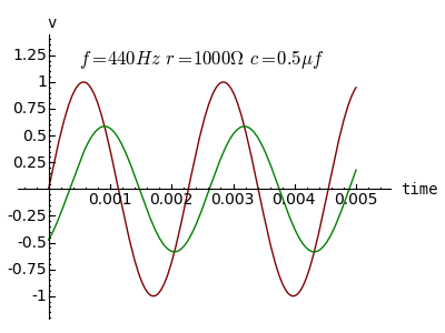
Notice the amplitude and phase relationship between the signal measured at the generator (red) and that measured at the capacitor (green). This is exactly what one would expect to see in an RC circuit — the capacitor's voltage peaks at the moment the driving waveform voltage matches that of the capacitor. In the same way, the tidal height in a bay peaks just as the ocean tidal height matches the bay's water level. This solution has many practical uses, including predictions of time and height for high and low tides in a bay connected to to the ocean by a channel.
This page shows some of Sage's power in addressing some real-world problems expressible as differential equations. It wsn't very long ago that such problems were out of reach of all but a few, in terms either of understanding or application. It is my hope and expectation that programs like Sage will create a revolution in math interest and education among people who might until now have regarded mathematics as an esoteric pursuit with few practical connections.
Such a revolution won't be predicated on the existence of computer algebra systems, because they've existed for several decades. The change will be based, not on the existence, but on the availability and ease of use, of math software. The tipping point will arrive when the everyday inconveniences produced by learning mathematics becomes a smaller burden than the everyday inconveniences produced by not learning mathematics.
"Exploring Mathematics with Sage" by Paul Lutus is licensed under a
Creative Commons Attribution-Noncommercial-Share Alike 3.0 United States License.
| Home | | Mathematics | | * Sage | | | | Share This Page |