Share This Page
| Home | | Mathematics | | * Applied Mathematics | | | Share This Page |
Approaches to managing storage tanks.
Copyright © 2012, Paul Lutus — Message Page
These pages address a key storage tank activity — creating a data table or equation that correlates sensor height measurements, for example dipstick readings or gauge indications, to the current volume of a tank's contents. This problem can be solved in one of two ways — through modeling and profiling:
Modeling means applying a mathematical equation that represents a geometric model of a storage tank (this is how TankCalc obtains its results).
Dimension Profiling means creating a tank outline or profile and mathematically modeling the tank on that basis. TankProfiler is the tool of choice for this method.
Content Profiling means applying a mathematical regression method to a set of direct sensor height and content measurements acquired from a storage tank whose dimensions are unknown. The best tool for this case it TankFlow.
Each method has its place, but modeling is overall a better approach — less effort and more accurate results. If your tank has a simple geometric shape, and if you can acquire the tank's dimensions and orientation, you should consider using the modeling approach — you should submit the tank's dimensions to my program TankCalc. This approach requires little effort, and the results are usually reliable.
If your tank doesn't have an easily defined shape, but can be measured and a dimensional profile can be acquired, the dimensional profile method is probably the best approach — see TankProfiler.
If, on the other hand, your tank's dimensions are not known, or if it has objects or protrusions inside it, or if it has changed shape for one reason or another, factors that prevent application of a simple mathematical model, you should consider the content profiling approach.
At first glance the reader may wonder whether the content profiling approach is ever required — most storage tanks fit into a small handful of geometric categories, and most are accessible to field measurements, so there's no reason to collect gauge/dipstick data over time to try to profile the tank. But in the years since I first wrote on this topic, and since I first released TankCalc, I have heard from any number of tank farm operators who asked about analyzing tanks that had "special problems."
Often an inquiry would describe a tank with a pathological shape, or a tank with internal protrusions or objects, or an underground tank that had never been measured and whose dimensions are unknown. For these cases, modeling just won't work — content profiling is required.
So, before we go on, a piece of advice — if you can get your tank's dimensions and there isn't anything preventing use of a simple mathematical model, I recommend that you visit the TankCalc page and enter your tank's dimensions — that's a much easier and more accurate tank evaluation method.
If you cannot get your tank's dimensions, or if there is something that prevents application of a simple model (like an object inside the tank that displaces content), or if the tank is buried and has an unknown shape or orientation, content profiling is the best approach.
The drawback to the content profiling approach is that direct content measurements must be taken at the tank — the tank must be drained and then filled in a controlled way, with a known flow rate over time, and sensor height measurements must be taken as the tank fills. For a large tank, in a busy yard, this can be a daunting task.
Again, be sure to visit the TankFlow home page to see a more in-depth practical discussion of this method.
The good news about this approach is that, once a set of measurements has been acquired that correlates tank volume with content height, the data can be converted into a special mathematical function that will reliably produce a partial volume for any sensor height argument. The general name for this method is "regression" or "regression analysis", and it has two primary forms:
Polynomial regression. This method produces a well-behaved mathematical function that relates sensor heights to content volume, based on a relatively small number of actual tank measurements. This approach works best when the original measurements are conducted carefully and the tank's shape isn't too pathological.
Here is a graph that shows the relationship between a handful of tank measurements (red dots) and the polynomial function's resulting prediction (blue line):
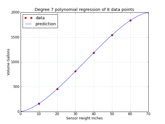
Figure 1: Polynomial regression result, 8 data points
The important thing to understand about polynomial regression is that, if the field measurements are carried out carefully, a very good profile of the tank can be acquired with only a handful of data points. In this case, the original data set is from a TankCalc model of a typical storage tank. Even though there are only 8 data points, the resulting correlation profile is very good, and can be used to accurately predict intermediate values:
Sensor Height True volume Profiled volume 0 0.00 0.00 5 56.54 57.75 10 162.30 162.30 15 298.50 298.40 20 456.34 456.34 25 629.35 629.37 30 812.09 812.09 35 999.60 999.59 40 1187.10 1187.10 45 1369.85 1369.82 50 1542.86 1542.86 55 1700.69 1700.80 60 1836.90 1836.90 65 1942.66 1941.44 70 1999.20 1999.20 Table 1: Comparison of measured data and polynomial regression
Linear interpolation. This method is very simple, essentially drawing a line between pairs of tank measurements and estimating the result on that basis. In most cases it is less accurate than polynomial regression, but it's very simple to compute and is suitable if high accuracy is not a requirement.
Here is an example of a linear interpolation (blue line) based on the same tank data set described above (red dots):
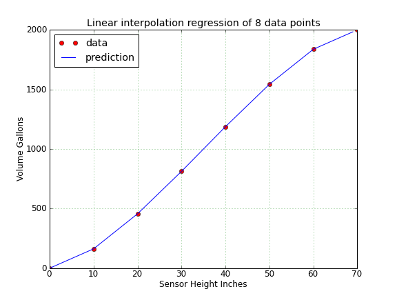
Figure 2: Linear interpolation result, 8 data points
Because this method draws straight lines between data points, it doesn't deal with curved surfaces very well. Note the relatively large errors in the table below for measured heights 5 and 65 — these are the tank locations having the greatest curvature:
Sensor Height True volume Profiled volume 0 0.00 0.00 5 56.54 81.15 10 162.30 162.30 15 298.50 309.32 20 456.34 456.34 25 629.35 634.22 30 812.09 812.09 35 999.60 999.60 40 1187.10 1187.10 45 1369.85 1364.98 50 1542.86 1542.86 55 1700.69 1689.88 60 1836.90 1836.90 65 1942.66 1918.05 70 1999.20 1999.20 Table 2: Comparison of measured data and linear regression
Notice about the two results above that the measured points were located at multiples of 10 inches (10,20,30 ...) (the location of the red dots in the graphs). Both tables (polynomial and linear), with steps of 5 inches, show their greatest accuracy at points that are multiples of 10. Remember this for future reference — when using these regression methods, a prediction that happens to fall on or near one of the original measurement points is likely to be essentially perfect (assuming the original measurement is). It is between these points that the polynomial method shows its superiority over the linear method.
Both the methods above can be used to generate a table that relates content height and volume, or to acquire a prediction for a specific sensor height. In other words, these methods can be used to create profile-based results similar to those TankCalc provides for modeled tanks.
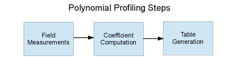
Polynomial profiling (or regression) is a reliable mathematical method that, when used to analyze a storage tank, has three phases:
- Taking sensor height readings as a tank fills at a known rate, and creating a table of raw data correlating sensor height with volume.
- Performing a mathematical procedure that converts the data table into a list of polynomial coefficients used in the next step.
- Producing results by way of a polynomial function mated with the list of coefficients computed in (2) above. In this step, we can produce either a table like that produced by TankCalc that correlates volume and sensor height, or we can submit single sensor heights to the function to get specific results.
To summarize, a relatively small number of field-measurement data points is used to create a table of coefficients, whicn in turn is used in a function to predict volumes for any sensor height, not just those measured:
(The comments in this section apply to both the polynomial and linear regression methods.)
This is the most difficult part of the profiling approach to storage tank analysis. It requires the most time, effort, and attention to detail, and it is why modeling a tank is much to be preferred to profiling one. Here are the steps:
- Drain the tank. This is essential for a tank whose content level is unknown or uncertain, and whose total capacity is unknown.
- Establish a reliable way to fill the tank, a method that will either deliver a constant, known rate of flow, or record the flow rate and time or each measurement. Ideally, a pump with a known flow rate connected to a large reservoir should be arranged.
- Make a log entry of the start time, and commence filling the tank using the costant-flow-rate source described in step (2) above.
- As the tank fills, periodically make log entries of:
(The more measurements, the better.)
- The time.
- The pump flow rate if it changes.
- The tank's sensor height reading.
- When the tank is full, stop the pump and mark the time and the final sensor height.
At this point it should be obvious why the source pump's flow rate must be known, and must either be constant or be recorded along with times and sensor heights. If the flow rate is not known, the tank's full capacity cannot be known. If the flow rate is not constant, unless the moment-to-moment flow rate is made part of the data collection, the intermediate sensor height measurements won't correspond to true intermediate volumes. For a usable result, both these uncertainties should be reduced or eliminated.
The above procedure should result in a log sheet having:
- A pumping start time, the time at which the tank was empty.
- Periodic entries with a time, a pump flow rate and a sensor height reading.
- A final tank-full entry with a time and a sensor reading.
Data Reduction
The purpose of this step is to convert the logged sensor height readings and times into a table of sensor readings and tank partial volumes. This task is most easily accomplished with a spreadsheet program to automatically convert times into elapsed times and thence into volumes, while avoiding clerical errors, but it can also be done by hand, with the assistance of a calculator. Here is the procedure:
For each logged measurement time, acquire an elapsed time by subtracting the start time from the measurement time, being sure to express the elapsed time in the same units that describe the pump's flow rate. Then multiply the elapsed time by the pump's flow rate to acquire a partial volume. Here is an example:
The above data conversion procedure is summarized in this equation — for each logged measurement:
- Let's say the pumping start time (st) was 14:22, and the pump's flow rate (fr) is 300 GPM.
- Let's further say that a measurement is taken at a time (mt) of 15:03.
- To convert from wall time to elapsed time, subtract 14:22 from 15:03 and express the result in minutes: 41.
- Multiply the elapsed time by the flow rate to determine the tank's partial volume at 15:03: 41 * 300 = 21,300 gallons.
- Make an entry in the result table. Include the partial volume computed above and the sensor height. Once the partial volume has been computed, the measurement time is no longer needed — only the sensor height and the partial volume appear in the result table.
- Repeat steps 2 through 5 above for each logged measurement.
(1) $ \displaystyle pv = (mt-st) fr $Where:
- pv = tank partial volume change during time interval mt
- mt = measurement time
- st = start time
- fr = pump flow rate
Be sure to use consistent units — if the pump's flow rate has units of gallons per minute, remember to express the elapsed time in minutes and the result volume in gallons. At the end of this procedure, you should have a table with two columns — one with sensor heights, and the other with partial tank volumes.
Practice Data Table
For this exercise, let's say we've used the above procedure to convert our field measurements into a table of sensor heights and volumes. Below is an example data table we'll use to practice generating coefficients in the next step:
Sensor Height Inches Partial Volume Gallons 0 0.00 10 162.30 20 456.34 30 812.09 40 1187.10 50 1542.86 60 1836.90 70 1999.20 Table 3: Example data set for coefficient computation
Polynomial coefficient computation is a relatively complex mathematical topic, but it's not necessary to understand it in order to to use it. In this step, we will take the practice data table listed above and submit it to my polynomial coefficient generator:
- Point your mouse cursor to the left of the first numeric row in Table 3 above (not the title row).
- While pressing the left mouse button, drag your mouse downward along the left side of the table.
- This action should cause the table's rows to be tinted, indicating that they're selected.
- Press the right mouse button and select "Copy".
- Click this link to open a new browser tab showing "Polysolve", my polynomial regression Web page.
- On the Polysolve page:
- Paste the clipboard contents acquired above into the window marked "Data Entry Area", replacing the sample data you will find there.
- Move to the "Degree" selector and use the arrow buttons to choose a degree of 7.
- At this point, you should see an S-shaped graph that resembles the graphs on this page, and below it, a table of 8 polynomial coefficients.
- Now select the "Table Generator" tab if it's not already selected.
- In the "Step" entry window, enter 5.
- Confirm that the "Decimals" entry (the number of result decimal places) is equal to 2.
- Confirm that the "Reverse" checkbox is not checked.
- Press the "Generate Table" button.
- A table of data should appear in the "Results Area" window. It should have this content:
x y % 0.00 0.00 0.00 5.00 57.75 7.14 10.00 162.30 14.29 15.00 298.40 21.43 20.00 456.34 28.57 25.00 629.37 35.71 30.00 812.09 42.86 35.00 999.59 50.00 40.00 1187.10 57.14 45.00 1369.82 64.29 50.00 1542.86 71.43 55.00 1700.80 78.57 60.00 1836.90 85.71 65.00 1941.44 92.86 70.00 1999.20 100.00 Table 4: Coefficient generation exercise result
- If the above result is confirmed, you have successfully rehearsed the process of processing field data, using them to create polynomial coefficients, then creating a tank profile result table.
- UPDATE: Because TankFlow now exists to assist in data reduction, this procedure is now much simpler then when this article was first written.
A bit more about Polysolve:
- When computing coefficients, it's normal to select a polynomial degree equal to the number of measurements minus 1. Example 20 measurements, degree 19. But this doesn't always work — if the measurements are scattered about because of systematic errors, the resulting graph may have twists and turns that reduce the predictive value of the result. In a case like this, decrease the degree of the conversion and examine the resulting graph. In the final analysis, a person looking at the graphed result is the best judge of quality.
- You may want many more data points in your result table than the automatic setting (which produces 20 rows). To accomplish this, simply decrease the step size in the "Step" entry to suit your requirements.
- You may need a table that relates volumes to sensor heights, the reverse of the above table, with evenly spaced volume values in the left-hand column producing sensor height values in the right-hand column. To accomplish this, simply check the "Reverse" checkbox. The "Reverse" mode switches all the data pairs (x,y -> y,x), which means the resulting table will predict sensor heights for provided partial volumes.
- The data table format has been chosen to be compatible with spreadsheet programs. In most cases it should be straightforward to use the system clipboard to import your table into a spreadhseet program for further processing and printing.
- After generating a table, you may want to see the polynomial result data again. To do this, press the "Solve" button.
- Some users may prefer to write their own computer programs to generate tank results based on the generated polynomial coefficients — for this purpose, Polysolve creates example functions for C/C++ and Java that incorporate the coefficients. To create these special results, press the "Form" button.
- Polysolve is available as a desktop application as well as a Web-based applet, with some operational advantages:
- Click here to download Polysolve as a Java desktop application JAR file for standalone operation.
- Click here to download the GPL-licensed source code archive for Polysolve, organized as a Netbeans project.
- You will need a Java runtime engine to use Polysolve as a desktop application. Click here to get a free Java runtime.
In actual practice, after using Polysolve to generate a data table, you would then copy the table into a spreadsheet or another editing environment for adjustment and printing. For example, you might want to change the column headings from "x" and "y" to "Sensor Height" and "Partial Volume", including the appropriate units.
Remember that you can create both sensor height -> volume and volume -> sensor height tables (and functions) with the same set of field measurement data, by simply checking the "Reverse" checkbox.
I include this section only for completeness — the polynomial regression method above is to be preferred in nearly all cases.
Again, linear interpolation predicts arbitrary data points by interpolating between measured data points. It does this by drawing a straight line between two adjacent data points and computing an intercept point for the provided coordinate.
There are some limitations to this method. One is that arguments must lie within the range of measured data points, they cannot fall outside. Another is that this method won't produce very good results if the original data shows any significant curvature between data points, something the polynomial method is better able to handle.
Rather than provide a lengthy tutorial as I did above, because of this method's limited usefulness, I offer this Python script (released under the GPL) that performs all the required colculations and table generation activities.
I apologize for the strict legalese below, but the calculations described here may be used to design and maintain fuel tanks and the possibilities for litigation have not escaped my attention. Sorry. Disclaimer of WarrantyThe computations and methods described here are provided on an "as-is" basis, without warranty of any kind, including without limitation the warranties of merchantability, fitness for a particular purpose and non-infringement. The entire risk as to the quality and performance of the computations is borne by you. Should the results prove to be in error, you assume the entire cost of any required service and repair, and any consequential damage.Limitation of LiabilityAs customary in the computer business, you are solely responsible for any loss of profit or any other commercial damage, including but not limited to special, incidental, consequential or other damages. This disclaimer specifically disclaims all other warranties, expressed or implied, including but not limited to the implied warranties of merchantability and fitness for a particular purpose, related to defects in the computed results or the documentation.
| Home | | Mathematics | | * Applied Mathematics | | | Share This Page |