To navigate this multi-page article:

Use the drop-down lists and arrow icons located at the top and bottom of each page.

 

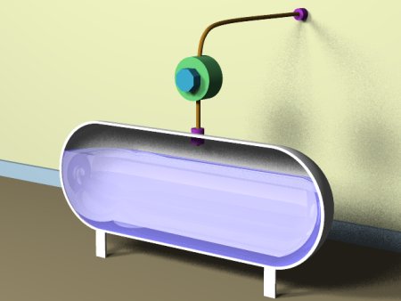Figure 1: Propane storage tank cutaway view

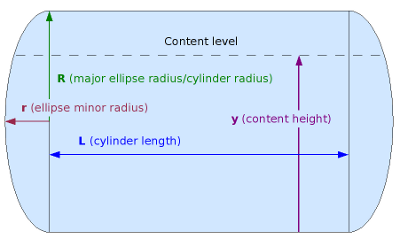Figure 2: Cylindrical tank variable names

This page describes methods for computing partial volumes in storage tanks such as are shown in Figures 1 and 2. This very common storage tank class includes simple cylinders with flat ends, cylinders with hemispherical ends, and many intermediate types with elliptical end caps (Figure 2). The methods on this page are suitable for computing partial volumes of all such tanks, with the single requirement that the tank be level.

For those who require analysis of a tank that is tilted, I recommend TankCalc, which knows how to compute this case.

As with many of this article's pages, this one serves two purposes — it is both a Sage tutorial and an applied-mathematics resource for those who need to compute tank volumes.

In reading this article it will benefit the reader to have access to a Sage notebook interface, either locally or online. To get your free copy of Sage, click here.

This class of tank is analyzed in two phases — the central cylindrical part, and the end caps — and the results are summed for a volume result.

(Click here for a Sage worksheet with resources used in this page.)

We're going to methodically work up to computing the kind of cylindrical tank shown in Figure 2, but we should first build a mathematical foundation. My approach to analyzing these tanks relies heavily on Calculus — in Integral Calculus we can take a relatively simple method that works in one dimension and create a solution that works in three. That is the basis for the method to be presented.

First, let's set up a Sage worksheet to accept what is to follow. Run Sage and open an empty worksheet. Copy the content below and paste it into the topmost cell of the sheet (or download this copy of my worksheet):

#auto
reset()
# special equation rendering
def render(x,name = "temp.png",size = "normal"):
    if(type(x) != type("")): x = latex(x)
    latex.eval("\\" + size + " $" + x + "$",{},"",name)
var('a d v R r y L')
forget()
assume(R >= 0)
assume(r >= 0)
assume(L >= 0)
assume(y >= 0)
            

Remember when copying and pasting these complex cell contents: resist the temptation to "fix" the indentation of certain lines. The indented lines must remain as shown for the content to work as intended.

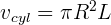
Moving on — the goal is to compute a cylindrical tank's content partial volume if given the tank's dimensions and a sensor reading. The sensor is typically a floating device in a tank containing liquid — the sensor provides the height of the tank's contents. Looking at Figures 1 and 2, it occurs to me that a good first step would be a function that provides a tank's width at any given sensor height y. Here is such a function:

dcyl(y,R) = 2*sqrt((2*R-y)*y)
render(d == dcyl(y,R),"equ_dia_cyl.png","large")
            

(1)  

Where: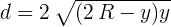

• R = tank radius.
• y = sensor height (0 <= y <= 2R)
• d = tank diameter at height y

To be sure this function does what we think, let's create a graph correlating sensor height y and the tank diameter our function predicts:

plot(dcyl(y,10),(y,0,20),figsize=(4,2.5))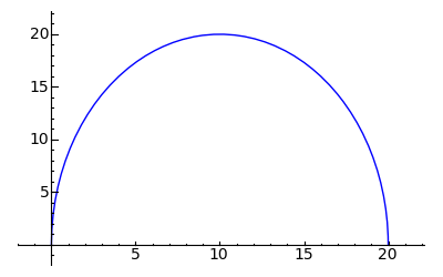

That looks reassuring — it's definitely the profile of a half-circle, and the value at y = R is the tank's diameter of 20 units. Now let's take the integral of "dcyl(y,R)" so we have a function we can use to compute partial circle areas:

vcyl(y,R,L) = ((integrate(dcyl(y,R),y)) * L).full_simplify()
render(v == vcyl(y,R,L),"equ_vol_cylinder1.png","large")
            

(2)  

Notice that I multiplied the integration result by L, to complete the partial volume of a cylinder. Let's graph this function and see if it produces valid partial areas for different y values:

plot(vcyl(y,10,1),(y,0,20),figsize=(4,3))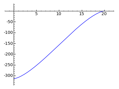

Okay, this is an an anomalous result — the integration produced a function that yields a range between -πR² and zero for a y range from zero to 2R. That's not what I expected from the original function or based on results derived from other programs. On the other hand, the canonical description of indefinite integration includes a constant of integration that must be accounted for:

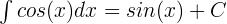
Where C is a constant that must be accounted for. Here's what Mathematica produces when presented with the same integration:

Here is a graph of the Mathematica result:

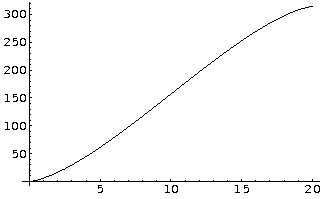
Okay, I think I'll provide an explicit constant of integration rather than try to find out why "integrate()" is doing this. Here's my adjusted integral:

vcyl(y,R,L) = ((integrate(dcyl(y,R),y) + pi*R^2) * L).full_simplify()
render(v == vcyl(y,R,L),"equ_vol_cylinder2.png","large")
            

(3)  

Notice that I added a term equal to "πR²", to correct the resulting range. Let's plot this new version of the function:

plot(vcyl(y,10,1),(y,0,20),figsize=(4,3))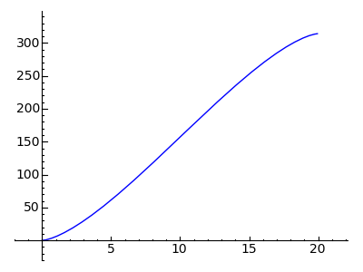

That looks correct. Given what this function models, one would expect to see an s-shaped curve, reflecting the fact that the rate of change in tank volume is greatest in the middle of the y value range and diminishes toward the top and bottom of the range.

Finally, a simple test: does this function produce the expected volume of a cylinder:

(4)  

vcyl(20,10,10)

1000*pi

The described cylinder has a radius of 10 units and a length of 10 units, and the y argument is equal to 2R (so the function provides a full volume), so this result seems correct.

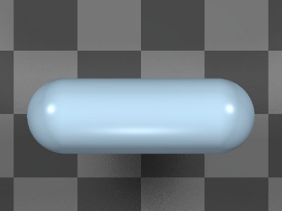Figure 3: Typical Propane Storage Tank

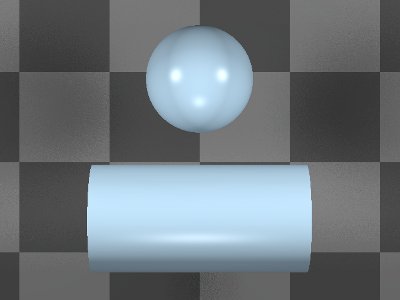Figure 4: Equivalent Volume: Cylinder + Sphere

Before we go on, a word about unification. The previous section's volume function assumes a y argument in the range 0 <= y <= 2R, to agree with its application in interpreting tank sensor readings. This section of the project represents a way to compute partial volumes of the tank's end caps, but it would be very useful if this section's use of the y content height argument would agree with that of the previous section, so the two separately computed elements (cylinder and end caps) may be unified into a single function for the entire tank, under control of the same variable.

Another important point about this tank type is a conceptual simplification — a cylindrical tank with a hemispherical cap on each end is equivalent in volume to a full sphere added to a cylinder, e.g. the two end caps can be analyzed as though they were a separate spherical or elliptical object that just happens to be split in two and occupies positions on the ends of a cylinder (see Figures 3 and 4).

As it turns out, an optimal way to proceed in this section is to create a function that produces circle areas for y arguments, as though we are slicing horizontally through a sphere at the height represented by y. Here is such a function:

acaps(y,R) = pi*(2*R-y)*y
render(a == acaps(y,R),"equ_area_caps.png","large")
            

(5)  

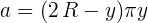
This should look familiar — it's a version of the equation used above to get cylinder widths. In the previous embodiment, a square root was taken to turn a surface area into a diameter. In this case we want a circle's surface area, so we eliminate the square root and multiply by π.

Let's integrate the above function to get a partial volume for a sphere bisected by y:

vcaps(y,r,R) = integrate(acaps(y,R)*r/R,y)
render(v == vcaps(y,r,R),"equ_vol_caps.png","large")
            

(6)  

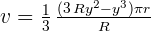
Astute readers will notice an added term in this function. The ratio r/R takes into account the minor radius of the elliptical end caps (see Figure 2 above), and it's used to adjust for end caps that are neither flat (in which case r = 0) nor fully spherical (in which case r = R). Here are the tank's computation variables at this stage (and refer to Figure 2 on this page):

• R = tank cylinder radius and end cap major radius.
• r = end cap minor radius.
• y = sensor measurement height, range 0 <= y <= 2R.

Later on when we combine the results for the cylinder and the end caps, we will see how these variables function together to produce consistent results (and by using consistent names we make it easier for Sage to simplify the expressions in which they appear).

Here is a graph for the end cap volume function:

plot(vcaps(y,10,10),(y,0,20),figsize=(4,3))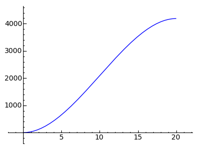

That looks right. Now one more test — we know that the volume of a sphere is equal to:

(7)  

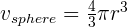vcaps(20,10,10)

4000/3*pi

That result for a sphere of radius 10 looks right also.

It would be nice to have a single function for partial volumes of the entire tank, one that combined the above separate results for the cylindrical section and the end caps. Here is an expression that combines them:

vfull(y,r,R,L) = (vcaps(y,r,R,L) + vcyl(y,R,L)).full_simplify()
render(v == vfull(y,r,R,L),"equ_vol_full.png","large")

(8)  

In this case, the Sage function "full_simplify()" greatly simplified the equation (not always true). Here's a graph for this function:

plot(vfull(y,3,5,10),y,0,10,figsize=(4,3))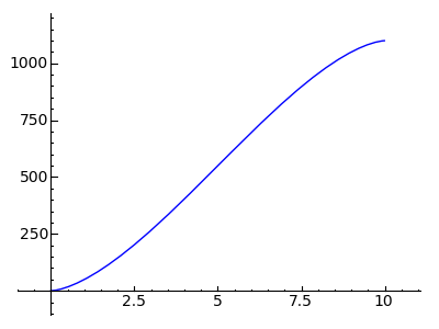

Testing the function

We should test our unified volume function by comparing it to a known value. As it turns out, for this tank type (and referring to Figure 2 on this page for variable names), a full volume is easy to establish. It's equal to:

(9)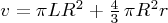  

Let's get a result from the combination function for a tank with these dimensions:

• L = 31
• R = 13
• r = 7

According to equation (9) above, we should get a result of (21414.14272...). Here's the result for our function:

N(vfull(26,7,13,31))

21414.1427244192

Obviously this function could be further tested using automated methods, but there is one property not trivially derived from other sources, and that is the partial volumes that are this function's purpose — that property is hinted at by the graph above showing the characteristic s-curve of partial volumes.

Some notes on this function:

• For a simple cylindrical tank with flat end caps, set r = 0.
• For a tank with spherical end caps, set r = R.
• For a spherical tank (with no central cylinder), set L = 0.
• The y argument range should always lie in the range 0 <= y <= 2R.

In this case, Sage's "simplify()" and "full_simplify()" functions were beneficial in combining and simplifying expressions. I've seen cases where they didn't significantly change the target expressions, and in a handful of cases the result was larger than the original. In one case to be described later, using "full_simplify()" instead of "simplify()" created a function that produced erroneous results - in other words, the result went beyond simplification into wholesale rewriting.

But the simplifications on this page may merit a closer look. Examine this equation:

(10)  

Notice the term "1/3" at the left. Now notice the constant multiplier "3" within the parentheses, a term that multiplies the entire dividend. Doesn't it seem reasonable that 3/1 and 1/3 should cancel out? I've seen a number of examples like this in Sage. I originally suspected this reluctance to combine terms arose from some restrictions having to do with complex numbers, but then I performed this test:

render((y/(3*x)).full_simplify(),"equ_simplify_fail.png","Large")

Hmm, that's odd. According to my lights, turning:

into:

doesn't count as simplification. I'm sure this must arise from my ignorance of higher mathematics. But here's how Mathematica handles a similar case:

Simplify[1/3 y/x]

Don't get me wrong — Mathematica is the enemy and costs about US$3000.00 besides (2009). But I suspect this is a bug in the "simplify()" algorithm, not something intentional (this discussion refers to Sage version 4.1.2).

  "Exploring Mathematics with Sage" by Paul Lutus is licensed under a
Creative Commons Attribution-Noncommercial-Share Alike 3.0 United States License.