

 Share This Page
| Home | | Computer Graphics | | | | Share This Page |
A creative Blender graphics project
— P. Lutus — Message Page —
Copyright © 2019, P. Lutus
Most recent update:
(double-click any word to see its definition)
Figure 1: Rotating Earth video. Click to start/stop.
First, some context. In this article, Blender refers, not to a kitchen appliance as some might assume, but to a terrific, free graphics workshop, a creative computer playground.
In this article I'll show how to use Blender to make a plausible rotating planet, with the option of stars in the background (actual astronomical stars!), shadows from terrain features, and other realistic touches. I include details and data sources for Earth, the Moon, and Mars.
This project moves forward in several stages:
- Learn how to make a smooth sphere.
- Learn how to decorate the sphere with appropriate map/terrain colors (different for Earth, the Moon, and Mars) and altitude data (with mountains/craters that cast shadows).
- Learn how to animate the result.
Fortunately, these steps happen to progress from easy to more challenging.
All the Blender files and instructions in this article are for Blender 2.80 and newer. On the topic of files, here's a link to the Blender file for the animated Earth model in Figure 1 (it requires an Earth surface details file described below).
This is an intermediate-level Blender project. But don't let that scare you — you can always download the Blender project files I provide and, by browsing around, figure out how things are done.
In this section we'll tackle the easiest parts. But first, let's take a look at Blender's user interface (Blender 2.80):

Figure 2: Blender basic layout (click for full size)
- The 3D Viewport is a sort of visual workshop, where you can add and remove things from your scene.
- The Outliner is a hierarchical diagram of your project that shows the relationship between elements of a scene.
- The Properties Editor gives you access to many kinds of controls, for display, animation, appearance of objects, and much more.
- The Timeline can be expanded and shows video sequencing and animation controls. It allows you to configure motions and property changes over time.
Some additional notes:
- The Blender user interface is very customizable, some might say to a fault, so back up your work regularly to be able to recover from an error.
- This project has several stages, each of which builds on what came before, so saving your work has particular significance, in particular because you can save a project file under a new name to preserve additions and changes.
- Remember that you can undo an action with keyboard shortcut Ctrl+Z, and "re-do" an "undo" with Shift+Ctrl+Z.
If things get confusing later on, refer back to this diagram for an overview.
Now we can get started!
Basic Sphere
- Run Blender and create a new, empty workspace.
- Select and delete the default cube.
- Choose menu item "Add" (keyboard shortcut: Shift+A) near the top of the 3D Viewport, then choose "Mesh", then choose "UV Sphere" — not "Ico Sphere". You should see this:
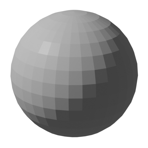
Figure 3: Unmodified UV sphere.
- Remember that Blender builds everything from polygons, like the little squares you see in Figure 3. There are many ways to avoid the aesthetic problems these polygons cause, but for now ...
- ... Click the sphere so it's selected (orange outline), then right-click it and choose "Shade Smooth". Now you should see this:

Figure 4: "Shade Smooth" sphere.
- One can also solve the polygon problem by increasing the number of segments and rings used to build the sphere, but the result draws and animates more slowly, something to be avoided. So "Shade Smooth" is the remedy of choice.
- Click here for the Blender file used to create the smooth sphere.
Equirectangular Images
We'll be using a special kind of graphic image to map a planet's features onto spheres. Such an image is called "equirectangular." An equirectangular image suitable for this project looks like this:

Figure 5: NASA Earth image from this website. This and related images are in the public domain. In NASA's words, "These images are freely available to educators, scientists, museums, and the public."
- Notice how the polar areas of the flat Earth image in Figure 5 are stretched horizontally. This is because those areas occupy less space on a globe. In fact, when mapped onto a globe the top and bottom of an equirectangular image represent almost no space at all.
An equirectangular image, although flat, is designed to map onto a globe and represent all latitudes accurately and in proportion. To see how this works, play this video:
Figure 6: Wrapping an equirectangular image onto a globe.
- Here is a link to the Blender file that created the video in Figure 6. Remember that to work as intended, this file needs to be provided with planetary surface color data (listed below).
Acquiring Resources
- The Blender file for Figure 6, and the next steps in this project, need two graphic images — one for earth's surface and one for the background stars.
- For the Earth surface detail image, choose from this list (different sizes of the NASA image described above), but be careful with the larger sizes — they can require some time to download and, when used by Blender, might require more memory than your computer possesses:
- The smaller background images are easy on your computer's memory and on Blender, but they don't produce very good Earth surface images because a full globe of detail requires a lot of data.
- Now for the Background star image. I created the image using a Python program I wrote, which reads a data table of nearly 120,000 stars from this website and creates an equirectangular image containing all the stars properly positioned.
- If the default 16000x8000 image (surprisingly small, 1 MB) I created is suitable, click here to download it.
- If the above image is too large, use this one instead (8000x4000, 900 KB).
- NOTE: These star background images are much larger in memory than when stored as files. A seemingly small image file may overwhelm your computer's memory when expanded for use.
- If you want to customize the image size, make it larger or smaller than the above choices, or choose different star rendering settings, you will need two things:
- My GPL-licensed Python script.
- A star database from http://www.astronexus.com/hyg, specifically this star database file (14 MB).
- The star database is licensed by a Creative Commons Attribution-ShareAlike license.
- If a custom star image is required:
- Unpack the database file and make it accessible to my script.
- In my Python program, choose settings to meet your requirements, then run the script to generate your own starfield graphic.
- The starfield image, equirectangular like the terrain map, is used as an environment background in this and my other Blender videos and still images.
- The starfield is accurate, the stars are real — here's a small segment of the full image:

Figure 7: Subset of equirectangular star image.
Click the image for more detail.- Those familiar with astronomy will recognize Orion in Figure 7, and the full-detail view acquired by clicking the image will reveal M42 located at the bottom center of the image.
- The background star image may seem unimportant as a background for an Earth image, but it makes more sense when we get to the Moon and Mars phases of this article.
Here's how to map the Earth surface detail image, acquired above, onto the sphere we created earlier:
- In the 3D viewport (refer to Figure 2), click the sphere so it's surrounded by an orange circle.
- Move to the Properties Editor at the lower right and, in the vertical row of tabs, locate and click the lower of two red globe tabs — choose the tab with the flyout text "Context: Material".
- The resulting pane should be blank except for a button saying "New". Click that button.
- Now you should have a new material on display that may be used to define the appearance of the sphere.
- In the list of properties, locate "Base Color" and a small circle to its right:

Figure 8: Locating the texture option
- Click the little circle and choose "Image Texture" from the options list that will appear.
- The original Base Color option will be replaced by an Image Texture option, including a file folder.
- Click the file folder and select your chosen image from the Earth surface detail image activity described above.
- In the 3D Viewport, locate the "Viewport Shading" buttons at the upper right. Choose "LookDev" mode, second from the right.
- Now you should see this:

Figure 9: Earth globe with surface details (click for full size)
In this step we'll create a Starfield Background for our planet.
- In the Properties Editor (refer to Figure 2), select the upper of two red globe tabs — choose the tab with the flyout text "Context: World".
- Locate the "Color" selector and, as before, notice the little circle to its right.
- Click that circle and choose "Environment Texture" from the options list that will appear.
- The "original "Color" option will be replaced by an Environment Texture option, including a file folder.
- Click the file folder and select a starfield image — you may want to review the Background Star Image activity above.
The star field won't yet be visible around the planet — a few more steps are needed:
- In the 3D Viewport, move to the upper right and select the "LookDev" option from the Viewport Shading option buttons.
- At the right of these option buttons is a down-pointing arrow — click it and select both "Scene Lights" and "Scene World".
- Move to the upper right of the 3D Viewport and toggle the perspective/orthogonal view (grid symbol) button — this should make the starfield appear around the planet.
Now let's test the result:
- On Planet Earth, are the continents in the correct orientation, or are they reversed left-to-right? If they're reversed, go back to the Earth surface detail image step above and repeat that step — choose an Image Texture, not an Environment Texture.
- Use the 3D Viewport navigation controls (upper right, X, Y and Z in different colors) to rotate the scene horizontally and bring the Orion constellation (see Figure 7) into view. Verify that your scene looks more or less like this:

Figure 10: Planet and Starfield (click for full-size view)
Notice Sirius, the brightest visible star*, directly below Planet Earth- If Orion is reversed left-to-right (refer to Figure 6), return to the Starfield Background step above and choose an Environment Texture, not an Image Texture.
- Hint: About the existence of two confusingly similar image formats — if the viewpoint is to be from outside the image, as with the planet's surface image, use an Image Texture. If the viewpoint is to be from inside the image, as with the star field, use an Environment Texture.
Here's a link to a Blender file for this phase of the project. Remember that it will need to be configured with the locations of the earth terrain and star field files listed above.
There's a lot of detail to animation, but for this example I'll make it as simple as possible. Be sure to regularly back up your work so you can recover from errors. And remember that Ctrl+Z is a convenient keyboard shortcut to "Undo" your most recent action. And Shift+Ctrl+Z "re-does" an undone action.
Above the 3D Viewport is a row of mode selectors: Layout, Modeling, Sculpting and so forth. Select "Animation" from this row of choices. This selection reconfigures the Blender user interface to allow easier animation activity. In particular, a new window opens below the 3D Viewport that's colorfully identified as the "Dope Sheet".
The Dope Sheet shows a time editor whose duration you choose depending on how long you want your animation to be. Below the Dope Sheet, a timeline should be visible, but if it's not fully in view, click the lower border of the Dope Sheet and move it up slightly. After this adjustment you should see:

Figure 11: Animation Setup (Click for full-size view)
Notice in Figure 11 that there is a timeline visible below the dope sheet. We need that timeline control to be able to set the animation's duration.
Now we can create an animation:
- In the Timeline (below the Dope Sheet), notice a control at the lower right with "Start" and "End" entries. Change "End" from its default of 250 to 360.
- At this point it may be necessary to adjust the Dope Sheet's size and layout so both the beginning and ending of the selected time range are visible. In Blender 2.80 and newer, the middle mouse button/scroll wheel accomplishes this — click the middle mouse button and drag to reposition the dope sheet's area, and spin the scroll wheel to change its size (i.e. zoom).
- If the Dope Sheet vertical blue control line isn't sitting on frame 1, move it there.
- Click our planet so it's surrounded by an orange circle.
- In the Properties Editor, choose the orange tab with the flyout text "Context: Object".
- Set the Z Rotation value to 0, then right-click this entry and choose "Insert Single Keyframe".
- Now move the Dope Sheet time control to frame 360, most easily accomplished by clicking the video control that commands a jump to the end of the range.
- Return to the Properties Editor, choose Context: Object, and enter a Z Rotation value of 359. As before, right-click this new entry and select "Insert Single Keyframe".
At this point, if you click "Play" or press the keyboard space bar, the animation should begin. Beginning slowly, then gradually speeding up, the planet will make one full rotation before slowing to a stop — then it will repeat the same sequence.
This gradual acceleration/deceleration, useful in animating moving objects, doesn't really work for a planet, so let's change it so the planet will rotate at a constant speed without speeding up and slowing down.
First, select all defined keyframes:
- At the beginning and end of the Dope Sheet time sequence you will see a vertical row of dots — those are the keyframes we defined earlier.
- While holding down the shift keyboard key, drag your mouse cursor across the keyframes, at both the beginning and ending of the Dope Sheet time sequence. This should make all the keyframes orange in color.
Now to change the keyframes' behavior:
- In the Dope Sheet's menu bar, select "Key".
- In the submenu that appears, select "Interpolation Mode".
- In that submenu, choose "Linear".
This change makes the planet move at a constant velocity, and if all the settings have been made correctly, the planet will rotate smoothly as the animation repeats (one rotation per animation sequence). The animation in Figure 1 of this article was created this way.
Click here to download the Blender file for this phase of the project.
All the methods explained earlier will be applied to the Moon (this section) and Mars (next section). But for the Moon and Mars there's an enhancement — a way to model altitudes and show terrain shadows, an effect that requires an extra data file. So for this model, three files are required:
- The Background star image from the prior section.
- A moon surface colors map.
- A terrain displacement map (with surface altitudes).
As before, for this project, all the files should be in equirectangular form.
Acquiring Resources
As it happens, shortly before this article was written, some dedicated people at the NASA Scientific Visualization Studio provided some perfect files for this specific application. This new project, named the CGI Moon Kit, offers a number of different resolutions and file sizes for both surface color and displacement.
Because I don't own these files, and because I want their creators to get the recognition they deserve, I'll instruct readers in how to download the needed files directly from their source.
NOTE: While choosing these files, remember that the larger files offer more detail, but require more memory and render more slowly.
- Go to the CGI Moon Kit website.
- Select and download one of the "Color Map" download options.
- Select and download one of the "Displacement" download options. For this project, download one of the files having "uint" as part of its name.
- The two files you download don't need to be the same size — different sizes work fine with each other.
Project Setup
This project is very much like the Earth model above, so we can re-use much of our prior effort:
- Run Blender and load the project file from the above animation activity.
- Save this project file under a new name to distinguish it from the Earth model.
- Switch the active workspace from Animation to Layout (top row of workspace choices).
- Click the planet sphere so it's surrounded by an orange circle.
- In the Properties Editor, select the "Context: Material" tab.
- In the Base Color definition, click the file folder and select the Moon Color Map file you downloaded in the prior step (this will replace the Earth surface image with the Moon surface image).
- If all goes according to plan, you should see this (with this Blender configuration file):

Figure 12: Moon without displacement data
Surface Displacement
Now to add surface displacement data. This step mixes two elements in the Moon image:
- Surface colors, already present as shown above.
- Surface displacement data, so that elevation differences will cast shadows.
Before we discuss the displacement modeling method, here's the result:
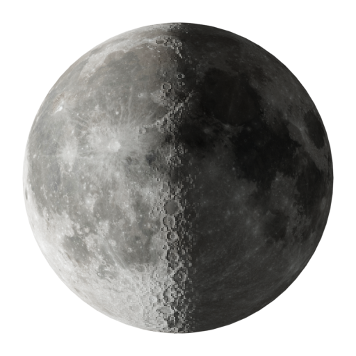
Figure 13: Moon with displacement data
Note the realistic shadows along the lunar terminator line (the point of lunar sunrise/sunset).
Here's a close-up comparison of lunar crater Tycho from our model, and a Lunar Reconnaisance Orbiter picture of the actual Tycho:
 Tycho: Blender
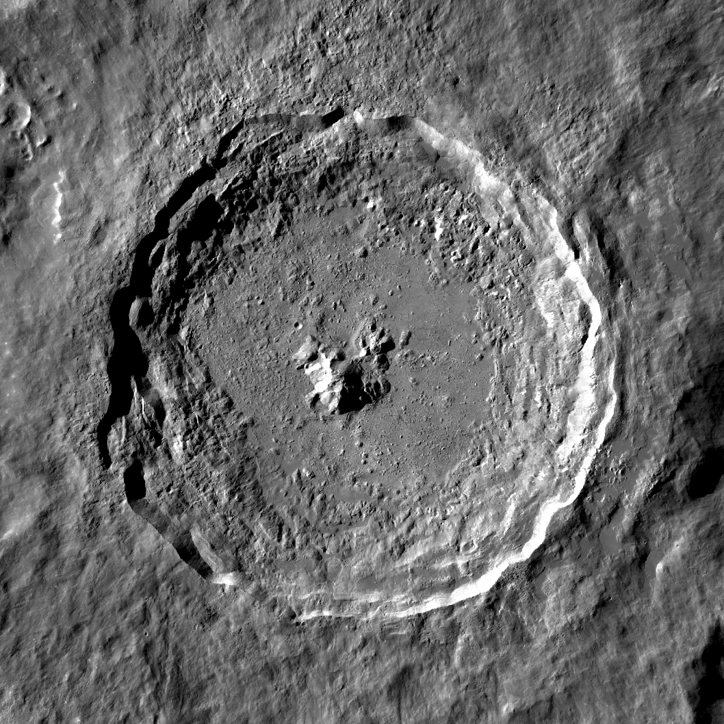 Tycho: LRO
Figure 14: Crater Tycho Comparison
Here's a video of some lunar terrain rendered using this method:
Figure 15: Lunar terrain video. Click to start/stop.
Before moving on, anticipating that the next phase and description may seem a bit technical and daunting, I suggest that readers click here for the Blender file that details the feature/altitude mixing method in Figure 16 (below), and click here for the Blender file that produced the video in Figure 15 (above). Remember about these files that, to work as intended, they need to be configured with surface color and terrain displacement data, available in this article.
Blender Material Configuration
The key to this method is to mix surface color and displacement data in a certain way, which requires that the Moon's Blender "material" be configured like this:

Figure 16: Moon material node diagram (click for full-size)
Here are the gory details:
- The Moon's material definition shown in in Figure 16 uses two Image Textures (orange top bars). One provides surface colors, the other provides displacement (altitude) data.
- The two Image Textures are synchronized with the sphere's polar coordinates by a Texture Coordinate node (red top bar at the left).
- The displacement data are converted into a usable form by a "bump map" node (purple top bar) — more on bump maps below.
- The amplitude of the displacement term needs to be carefully managed to avoid exaggerated shadows. This is controlled by the Bump Map's "Strength" control.
- The surface color data is provided to the primary BSDF (bidirectional scattering distribution function) (green top bar) node as a Base Color input.
- The Bump Map node provides data to the primary BSDF node as a "normal" input, "normal" in this context meaning surface angular deviation from the vertical.
- The primary BSDF provides its result to a Material Output node (red top bar at the right) for interactive display and rendering.
The result is that realistic surface colors and terrain shadows appear on the lunar surface as the sun's angle changes. People familiar with telescopic and spacecraft views of the moon will immediately recognize the details along the lunar terminator (i.e. sunrise/sunset) line.
Bump Map
A few words about the "Bump Map" node shown in Figure 16. The Bump Map converts altitude data into surface angles for the BSDF's "normal" input, so realistic shadows can be rendered. This scheme works reasonably well, but it's important to remember that the method doesn't create literal altitude variations on the sphere's surface, consequently even though a tall lunar mountain will have a realistic shadow, it won't cast a silhouette across nearby terrain.
An alternative drawing strategy would be to break the sphere into many small rectangles (more than is already true) and assign each vertex an altitude from the surface displacement data source. Although this can be done, it requires much more memory and processor speed than the "bump map" strategy. The result on a typical computer is unacceptably slow render times.
Readers may be able to guess that, at this point, creating a Mars model will be easy — all we need to do is copy the Moon model from above and change two data files — the surface colors file and the displacements file. These are the files required by the planetary material definition shown in Figure 16. So we need to find suitable Mars equivalents.
Surface Color
A good source for equirectangular Mars surface color images is this Wikimedia Commons site. Because these images are in the public domain, I've processed the largest image (included below) to create a range of sizes for different needs:
Surface Displacement (altitude)
A different source is available for surface displacement, at this USGS Astrogeology site. These images are also in the public domain, so as above, I've processed the original, very large image available at the site (2 GB in size, therefore not included here) to more reasonable dimensions and file sizes:
- 2048x1024 (44.4 KB)
- 4096x2048 (124.8 KB)
- 8192x4096 (349.8 KB)
- 16384x8192 (1 MB)
- 32768x16384 (14.1 MB)
Create The Model
Make a copy of the Blender Moon model from the prior example, save it under a new name, and replace the two files required by the planetary material nodes shown in Figure 16. With reasonable care you should soon have a Mars model like this one:
Figure 17: Mars terrain video. Click to start/stop.
Click here for the Blender file containing the Mars model. Remember that to work as intended, this file needs to be provided with planetary surface color and displacement (altitude) data files (listed above).
This article shows how to use Blender to create realistic, orbiting planetary models with surface colors and terrain relief, then animate them for added realism. The planetary data files required to support these models is free and available in many resolutions, some listed above in this article.
The Blender models can be examined and manipulated as part of education and familiarization exercises, and with some extra effort, made part of animated CGI productions.
Remember about this article's linked Blender files that each needs at least two additional data files — surface colors and terrain displacement (altitude) data — which are provided in each article section.
Thanks for reading!
| Home | | Computer Graphics | | | | Share This Page |
